Basic Time-Series Analysis: Model Choice Cookbook
This post is the sixth and final in a series explaining Basic Time Series Analysis. Click the link to check out the first post which focused on stationarity versus non-stationarity, and to find a list of other topics covered. As a reminder, this post is intended to be a very applied example of how use certain tests and models in a time-sereis analysis, either to get someone started learning about time-series techniques or to provide a big-picture perspective to someone taking a formal time-series class where the stats are coming fast and furious. As in the first post, the code producing these examples is provided for those who want to follow along in R. If you aren’t into R, just ignore the code blocks and the intuition will follow.
This post concludes the sequence of posts on time series basics. It certainly doesn’t replace the need for a good course in time-series econometrics/statistics; there are a lot of complicating factors and model extensions I didn’t touch upon. But, I hope beginners can use it to get started poking at their own questions, or reading others’ research based on little more than what is covered in these posts.
So with that, the final post in this series provides a ‘cookbook’ approach, or series of questions along a decision tree to guide you toward what kind of model you should be thinking about for your own analysis.
Cookbook for Model Selection
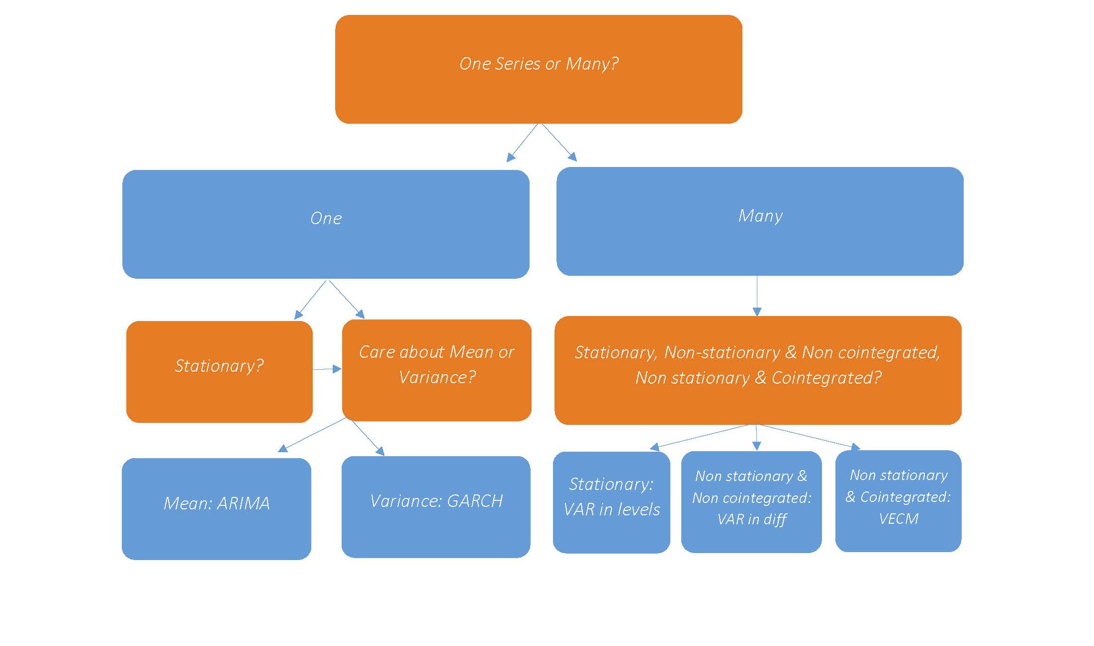
One minor detail. After deciding that you have one series you want to explore, you determine if the series is stationary or not. This flows into the Mean/Variance? box because whether or not the series are stationary partially determines the form the ARIMA or GARCH will take.
Links
Links to previous posts in this series are presented below for convenience.
- Stationarity
- ARIMA
- GARCH
- VAR
- Cointegration and VECM
- Cookbook for model Selection (current post)
Blogs
There are tons of great stats and time series blogs out there. Forgive me if I don’t link to your favorite (or the one you write!) But, there are a couple that stand out in my mind so I will link them here as resources to learn more. If I’ve overlooked any obvious gems, please post in the comments!
Dave Giles’ Econometrics Beat: This blog is one of the best and most widely read on the web. Dave gets down into the nitty gritty, much more so than I have done in this series. I learn something every time I take the time to read one of his posts. He doesn’t cover time series exclusively, but I believe the majority of posts are about time series topics.
Rob Hyndman’s Hyndsight Blog: In the blog itself, Rob doesn’t get into explaining econometrics too much. However, he has been one of the most prolific creators or R packages for time series and forecasting. His website is a good gateway to all of that material.
That’s It!
Well, that’s it for this series on the Basics of Time Series econometrics. Thanks for reading along!